Spatial analysis · retail site selection

Identifying Store Expansion Locations with Location Intelligence

Retail site selection is usually decided on intuition and partial information. This study replaces that with geospatial data enrichment and a revenue model, ranking every US metro region without a store and returning the twenty worth opening in.

Role: Sole analyst
Unit of analysis: Metro CBSA regions
United States
Features: 6 socioeconomic
& point-of-interest
Model: Random Forest regressor
100 trees · 80/20 split
Result: 0.83 test R²
Top 20 locations ranked

The problem

Choosing where to open a retail store is a hard question dressed up as a simple one. The answer depends on customer demographics, on where competitors already sit, and on what surrounds the site — and in practice the decision is often made on guesswork or on whatever information happened to be at hand. The alternative is to treat the question as what it actually is: a spatial one.

Objectives

Integrate and analyse geospatial and socioeconomic data to assess market potential across regions.
Train a model that learns the relationship between regional features and commercial performance, and use it to predict high-potential locations.
Visualise the results as maps, so the recommendation is legible to the people who have to act on it.

Workflow

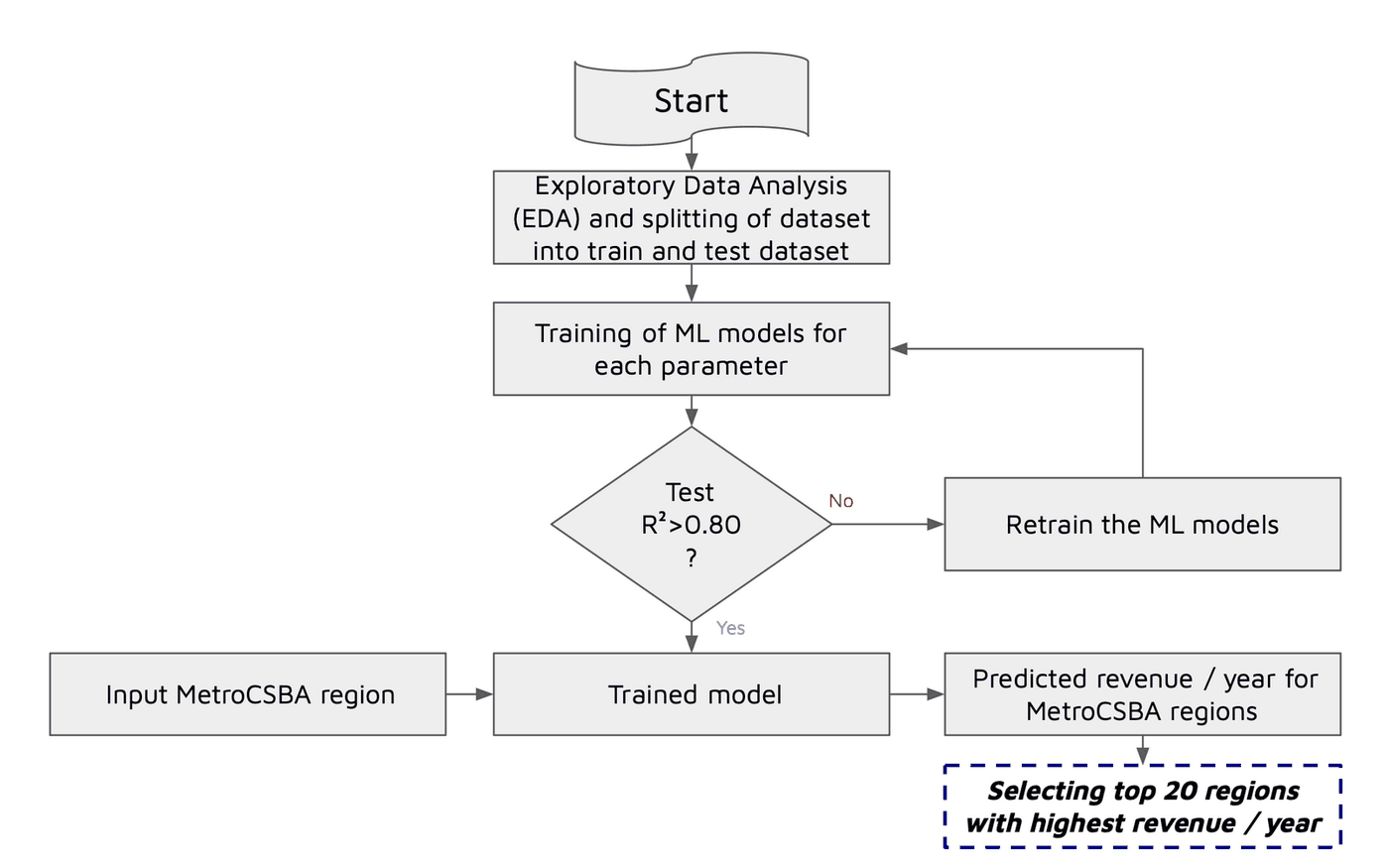
Five stages, from choosing what to measure through to naming the regions worth opening in.

01 FilteringSelect non-spatial attributes by deductive reasoning

02 EnrichmentSpatial join of point datasets onto Metro CBSA regions

03 AlignmentJoin independent and dependent variables into a training table

04 Machine learningTrain and evaluate on RMSE and R²

05 AllocationRank the top 20 regions by predicted yearly revenue

Data enrichment

The independent variables are a mix of census-style attributes and counts derived from point data. Colleges and universities, competitors and shopping centres arrive as individual locations, so each point layer is spatially joined onto the Metro CBSA polygons and aggregated to a per-region count — turning scattered points into a regional attribute the model can use.

Feature	Type	Source form
Median household income	Continuous	Regional attribute
Population density	Continuous	Regional attribute
Average (mean) age	Continuous	Regional attribute
College and university count	Count	Point layer, spatially joined
Shopping centre count	Count	Point layer, spatially joined
Competitor count	Count	Point layer, spatially joined

Methodology flowchart: exploratory data analysis, train/test split, model training, a test R-squared above 0.80 gate with a retrain loop, then prediction and selection of the top 20 regions — **Fig. 01**Modelling methodology. The R² > 0.80 gate sends the model back for retraining rather than letting a weak fit through to prediction.

Choosing the target

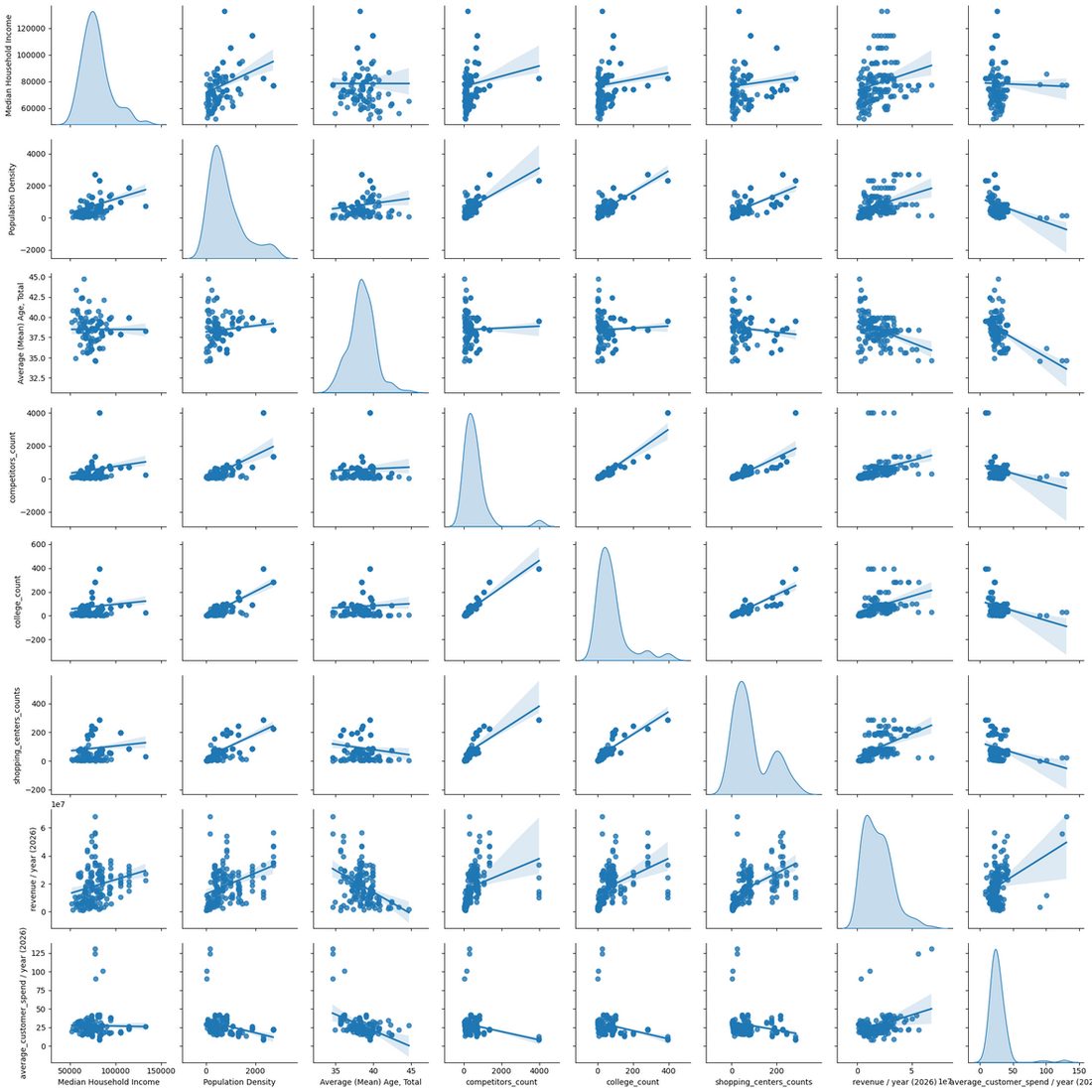
Two candidate target variables were available, and the exploratory analysis, not assumption, decided between them.

Average customer spend per year was rejected. Its correlation with the independent variables was weak and negative — there was no signal for a model to learn.
Revenue per year was selected. It correlated strongly and positively with the independent variables, which also served to validate the deductive reasoning that picked those features in the first place.

Two findings worth keeping

Average age correlates negatively with revenue — younger populations are associated with higher revenue, which is a directional result a site-selection team can act on directly.
Competitor count correlates positively with revenue, contrary to the initial expectation that competitors would depress it. Rather than discard the variable for disagreeing with the prior, it was retained — competitor presence appears to mark proven retail demand rather than saturated supply.

Pairwise scatter plot matrix of all model variables with fitted regression lines and kernel density plots on the diagonal — **Fig. 02**Pairwise relationships across all variables. The regression line in each panel is what drove target selection and surfaced the age and competitor findings.

The model

A Random Forest regressor with 100 estimators, trained on an 80/20 split. The methodology gates on test performance: a model that fails to clear R² > 0.80 on unseen data is sent back to be retrained rather than carried forward into prediction.

Metric	Score	Reading
Training R²	0.87	The model explains 87% of the variance in the training data, having learned the pattern between regional features and revenue.
Testing R²	0.83	Held up on unseen data, confirming the relationship generalises rather than being memorised. The narrow train-test gap indicates the fit is not overfit.

Results

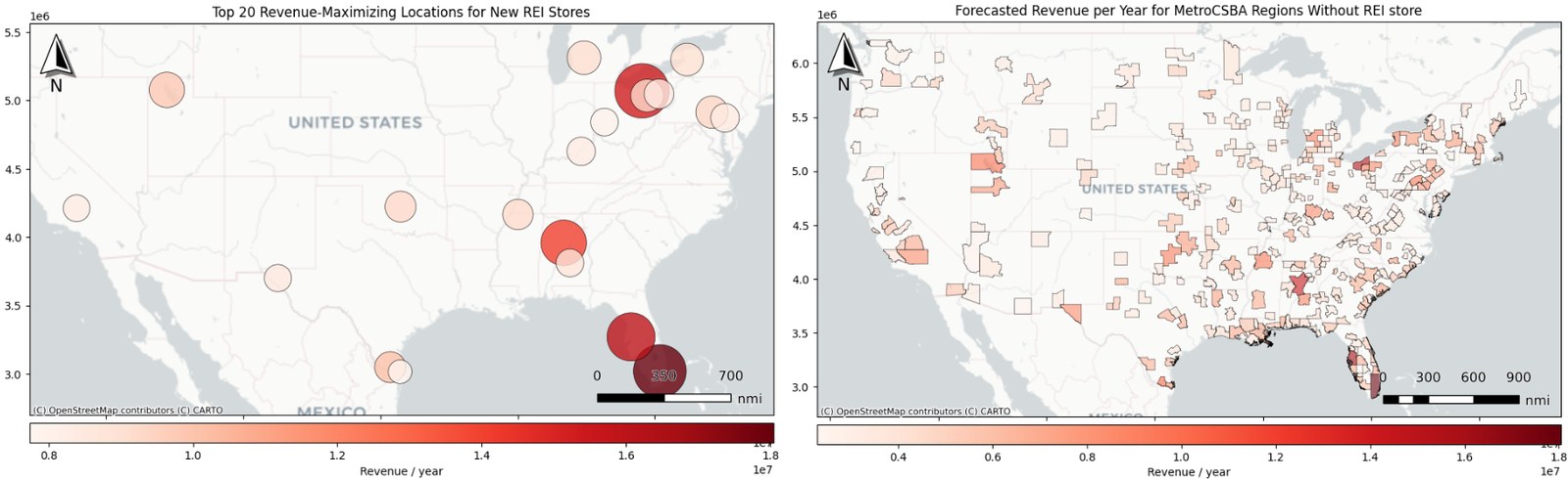
The trained model was applied to every Metro CBSA region that does not currently have a store, producing a nationwide forecast of the potential market rather than a shortlist assembled by hand. Regions across the Southeast, the Northeast and parts of the West forecast strongly, with several at $10M–$18M per year.

The final twenty were then selected from that full forecast by predicted annual revenue. They are geographically diverse, clustering in the Southeast and Northeast with the remainder spread across the West and South-Central states.

Two maps of the United States: the top 20 revenue-maximising locations for new stores, and forecast revenue per year across all metro regions without a store — **Fig. 03**Left — the final top 20 revenue-maximising locations. Right — forecast revenue across every metro region without a store, the full landscape the twenty were drawn from.

Conclusion

Combining location-based data enrichment with machine learning identified high-potential regions reliably enough to base an expansion shortlist on — the spatial join is what turns scattered points of interest into features a model can actually learn from.

Where it goes next

The current model treats each region as an independent row of attributes, which leaves the geography on the table. A spatially aware model — one that exploits the distribution of the data points themselves rather than only their aggregated counts — should capture location-based effects such as regional clustering and spillover between neighbouring markets, and improve predictive accuracy with them.

← Palm Tree Classification All work →